ВИЗУАЛИЗАЦИЯ ЭЛЕКТРОМАГНИТНЫХ ВОЛН С ПОМОЩЬЮ PYTHON

1. Introduction

Though unseen, electromagnetic fields—the dynamic relationship between electric and magnetic forces—are the driving power behind modern technology. They enable everything from the wireless networks that keep us connected to the vital magnetic fields used in medical imaging technologies such as MRI. These fields are essential in both physics and engineering. Central to our comprehension of electromagnetism is a collection of four equations developed by James Clerk Maxwell in the 19th century. These equations not only brought together the concepts of electricity and magnetism but also foretold the existence of electromagnetic waves, which laid the groundwork for innovations such as radio, television, and the internet.

Key Terms

Electric Fields: 

An electric field is a region of space where an electric charge experiences a force.

Magnetic Fields: 

A magnetic field is a region of space where a moving electric charge or a magnetic material experiences a force

Electromagnetic Waves:

Set of waves which propagate through space and carry momentum and EM radiant energy

2. Analyze of Maxwell's Equations and the Foundation of Electromagnetism

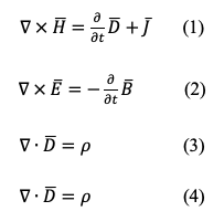
Electromagnetic theory explores the intricate dance between electric and magnetic fields, revealing how charges and currents generate forces and electromagnetic waves that propagate through space. At its core lie Maxwell's equations, four fundamental relationships that elegantly link electric and magnetic fields to their sources and to each other. These equations not only unified the previously disparate laws of electricity and magnetism—including Coulomb's, Gauss's, Faraday's, and Ampere's laws—but also unveiled the electromagnetic nature of light and all other forms of radiation. In 1873, James Clerk Maxwell (1831–1879) formalized these laws, presenting them in their complete three-dimensional vector form.

The Maxwell equations, in three-dimensional vector notation, are

Where  and ρ are real functions of position and time [2, p. 3].

Equation (1) is Ampere’s law with Maxwell’s equation or the generalized Ampere circuit law.

Equation (2) is Faraday’s electromagnetic induction law.

Equation (3) is Gauss’ law for electric fields.

Equation (4) is Gauss’ law for magnetic fields.

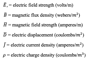
We generally refer to  as electric fields, and  as magnetic fields.

Maxwell’s contribution to the laws of electromagnetics is the term ∂D/∂t, which is called the displacement current. The addition of the displacement current to the electric current density J (r,t) in the original Ampere’s law has at least three major consequences. First, in a capacitor which is an open circuit for direct current, the displacement current ensures the continuity of alternating currents in electric circuits. Secondly, the continuity law

follows from (1) and (3) by making use of the vector identity  It is the displacement term that guarantees the conservation of electric current and charge densities. Equation (5) states that the electric current and charge densities are conserved at all time. Thirdly, Faraday’s law in (2) states that a time-varying magnetic field induces a circulating, time varying electric field. With the displacement term in (1), Ampere’s law states that around time-varying electric fields, time-varying magnetic fields are produced. This interrelationship between the time-varying electric and magnetic fields constitutes the foundation of electromagnetic wave theory and led Maxwell to the prediction of electromagnetic waves.

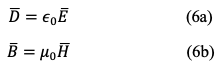
In developing his theory for the electromagnetic fields in space and time, Maxwell conceived of a substance filling the whole space called aether. In the aether, the electric fields   are related by a dielectric permittivity ϵ₀, and the magnetic fields are related by a magnetic permeability μ₀.

Where:

 

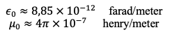
where the numerical values for ϵ₀ and μ₀ are expressed in MKS units. We now call (6) the constitutive relations for free space [3, p. 16].

3. Methodology

3.1 Purpose of the code:

We create a computer simulation that models the dynamics of the electromagnetic field in a vacuum. For this, the finite difference time domain method (FDTD) is used — one of the classical numerical methods in electrodynamics. In our case, we consider a two-dimensional situation (2D) for the TM mode (Transverse Magnetic, «transverse magnetic» mode), where the only non-zero component of the electric field is E_z.

Why is this important?

Maxwell's equations describe how electromagnetic waves (e.g., light, radio waves) propagate.

The FDTD method provides a numerical solution to these equations, which is useful in modeling physical processes and designing devices.

3.2 Normalize units:

In physics, SI units are often used (meters, seconds, Farads, Henry, etc.), but in numerical modeling it is convenient to use normalized units:

Why normalization?

When normalization, all quantities are reduced to dimensionless values, which simplifies calculations and avoids errors associated with very large or very small numbers (for example, the speed of light c≈3×10⁸ m/s in SI units).

Example:

If you have an equation  when standardized it becomes  which is much easier to calculate.

What's going on inside:

Three arrays are created:

Initializing the source:

A Gaussian pulse is created on the grid, which means that the values Ez​ in the center of the grid are installed according to the formula:

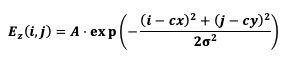
where:

A — amplitude,

σ — parameter that determines the pulse width,

cx, cy — coordinates of the canter of momentum.

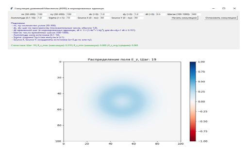
 Figure 1. Generation of a Gaussian Pulse

In Figure 1, we observe the generation of a Gaussian pulse in a two-dimensional grid, representing the initial disturbance in the electric field component Ez. The pulse is centred in the grid, with the highest amplitude at the centre and a gradual decrease toward the edges. The pulse is strongest at the centre (shown in blue) and fades toward the edges (warmer colours like red). This snapshot captures the starting point of our simulation, where we’ll track how the pulse evolves over time. It’s a vivid way to visualize the birth of an electromagnetic wave!

An example from life:

Imagine you spill a little paint in the center of a white sheet of paper – the paint intensity will be highest in the center and gradually decrease towards the edges according to a Gaussian distribution.

3.3 Magnetic Field Update H_x​ and H_y​

Update formulas:

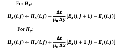
Explanation:

Δt — time step, shows how much the field changes in one step.

Δx, Δy — distance between nodes.

Expressions of the form [E_z(i,j+1)-E_z(i,j)] — this is a difference approximation of the derivative with respect to space, that is, a change E_z between two adjacent nodes.

Analogy:

This is like measuring the temperature difference between two adjacent rooms to see how much the temperature varies from room to room.

3.4 Electric field update E_z​

Update formula:

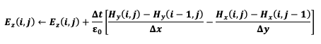
Explanation:

Here, difference approximations are used for the spatial derivatives of the magnetic field

The “+” sign indicates that Ez changes under the influence of the difference between changes in magnetic fields.

Example:

If we imagine that H_y and H_x — are water flows, then the difference in flows at adjacent points determines how the water level changes (analog  E_z).

3.5 Visualization with matplotlib

Creating a plot:

Using the Figure function from matplotlib library, we can create a plot. Then the imshow () function which allows us to render an image to a rectangular region in data space is employed to display the matrix E_z as a color map, where different colors correspond to varying field values.

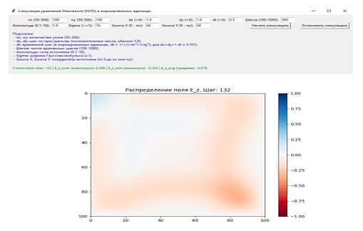
Figure 2: Electric Field Distribution

In Figure 2, the electric field distribution at time step 132 is visualized using a color map generated by the imshow() function from the matplotlib library. The color map represents the intensity of the electric field E_z across a spatial domain, with different colors corresponding to different field values. This visualization helps in understanding the spatial variation and strength of the electric field at a given time step.

Analogy:

It's like watching a movie, where each image is a frame showing how the distribution of paint on a sheet change over time.

Animation:

The animation aspect, facilitated by the matplotlib.animation.FuncAnimation class in python (A class used to make animation by repeatedly calling the same function), allows for the dynamic updating of this plot over successive time steps, providing insight into how the electric field evolves over time. This is particularly useful for studying wave propagation, electromagnetic fields, and other time-dependent phenomena in physics and engineering.

In our case it collects the data at each step then tabulates it. The table contains the following columns:

1. Step: time step number,
2. E_z max: maximum field value E_z,
3. E_z min: minimum field value E_z,
4. E_z avg: average field value E_z.

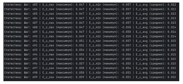
Figure 3: Part of the table showing the data collected for the last 17 steps.

4. Finite Difference Method (FDTD)

FDTD (Finite-Difference Time-Domain) is a numerical method that:

• Breaks space into a grid (discretization).
• Approximates derivatives using finite differences.
• Updates field values ​​step by time.

Visualization of Electromagnetic fields video:

https://disk.yandex.ru/i/NkzaSMI3o3s34A

Example:

If you want to calculate the rate of temperature change, you can measure the temperature difference at neighbouring points and divide by the distance between them. FDTD does a similar calculation for fields.

5. Boundary conditions

In numerical simulation, the domain is bounded (a set of nodes). Boundary conditions (e.g E_z=0E_z=0E_z​=0 at the edges) are used to simulate the situation where waves «disappear» outside the simulation area [4, p. 303].

For all fields, boundary conditions are set, where the field value at the edges of the grid is fixed equal to zero:

E_z(0,j)=E_z(nx-1,j)=E_z(i,0)=E_z(i,ny-1)=0

And similarly, for H_x and H_y.

Why is this necessary?

This is a simulation of absorbing boundaries so that waves do not reflect from the edges of the simulation area and do not disturb the dynamics inside.

6. Conclusion

This study has demonstrated the effective visualization of electromagnetic wave propagation through a Python-based implementation of the Finite-Difference Time-Domain (FDTD) method. By simulating a two-dimensional Transverse Magnetic (TM) mode in a vacuum, we have visually confirmed fundamental electromagnetic principles derived from Maxwell's equations.

The Significance of This Work:

Bridging Theory and Practice:

The simulation provides a tangible link between the abstract mathematical formulations of Maxwell's equations and the observable behavior of electromagnetic waves. For example, the visualization of the Gaussian pulse propagation directly illustrates the wave nature of electromagnetic energy, reinforcing theoretical predictions. Furthermore, the quantitative data generated by the simulation, the maximum, minimum, and average E_z field values, allows for a more in-depth analysis of the wave propagation.

This is crucial for educational purposes, allowing students and researchers to develop an intuitive understanding of electromagnetic phenomena.

Computational Electromagnetics and Its Impact:

The FDTD method, pioneered by Kane Yee in 1966, has proven to be a transformative tool in computational electromagnetics. Its ability to directly solve time-dependent Maxwell's equations has enabled the modeling of complex electromagnetic systems across various disciplines.

For instance, in telecommunications, FDTD simulations are essential for optimizing antenna designs, analyzing signal propagation in urban environments, and developing advanced microwave devices. In optics, FDTD is used to model photonic crystals, waveguides, and metamaterials, driving innovation in optical technologies. In radar, FDTD simulations are used for radar cross section calculations, and for the simulation of radar wave propagation in complex environments.

The increase in computing power has allowed for the FDTD method to be used on larger and larger problems, and is now used extensively in industry, and academia.

Python as a Powerful Tool for Scientific Computing:

This project highlights the versatility of Python as a platform for scientific computing. The combination of NumPy for numerical computation and Matplotlib for visualization provides a powerful and accessible environment for developing electromagnetic simulations.

The interactive nature of the Matplotlib animations allows users to observe the dynamic evolution of electromagnetic fields, enhancing their understanding of wave propagation. Furthermore, the use of python allows for rapid prototyping of electromagnetic devices.

Limitations and Future Directions:

It is important to acknowledge the limitations of this study. The two-dimensional TM mode simplification limits the complexity of the simulated scenarios. Future work should focus on extending the simulation to three dimensions to model more realistic electromagnetic phenomena.

Additionally, the use of simple absorbing boundary conditions could be improved by implementing Perfectly Matched Layers (PMLs) to minimize reflections. Furthermore, the simulation could be enhanced by incorporating dispersive materials and optimizing the code for performance using techniques like GPU acceleration.

Future work could also focus on developing more advanced visualization techniques, such as three-dimensional rendering and interactive manipulation of the simulation parameters.

Educational Impact:

This type of simulation has immense educational value, allowing students and researchers to visualize and explore electromagnetic phenomena in an interactive and engaging way. By providing a hands-on approach to learning, it can significantly enhance comprehension and inspire further exploration in the field of electromagnetics. The code that produces this simulation can be used as a teaching tool.

In conclusion, this research provides a valuable demonstration of the FDTD method and its application in visualizing electromagnetic wave propagation. By bridging theory and practice, and by highlighting the power of computational tools, this study contributes to a deeper understanding of fundamental electromagnetic principles and their relevance to modern technology.