INTEGRATED GEOLOGICAL MODELING OF TERRIGENOUS RESERVOIRS OF THE BOBRIKOVSKY HORIZON USING SEISMIC ATTRIBUTES AND GEOSTATISTICAL METHODS

Introduction

The Bobrikovsky horizon (C1bb) within the South Tatar Arch (Republic of Tatarstan) exhibits significant lateral and vertical variability of reservoir properties due to its alluvial deltaic and shallow marine origin [1, 3]. Conventional deterministic interpolation of well log data fails to accurately reproduce the geometry of sand bodies in inter well space, leading to high uncertainty in reserve estimation and field development planning [2]. A modern solution is the integration of well log and 3D seismic data using geostatistical methods and seismic attributes [6,7,9]. The aim of this work is to build a reliable 3D geological model of the Bobrikovsky horizon based on TGS facies modeling, collocated cokriging of porosity with acoustic impedance (AI), and Leverett J function saturation modeling, followed by volumetric reserve estimation.

Geological setting and input data

The study targets terrigenous deposits of the Bobrikovsky horizon (Lower Visean) in the South Tatar Arch. The section is dominated by quartzose sandstones (quartz content up to 99%), siltstones and argillites [1, 4 с. 46]. The horizon thickness ranges from 30 to 52 m. Lithofacies analysis defines two main facies: sandstone (reservoir) and shale (non reservoir). Sand bodies are lenticular with a preferred orientation of 75° azimuth, consistent with regional paleocurrent direction [3].

The study uses data from 41 wells with full log suites (gamma ray, neutron, density, resistivity), a 3D seismic cube (Inline 208 × Xline 805, time range 0–1000 ms), checkshot data for key well No. 73 for seismic to well tie, and petrophysical equations calibrated to core from the Bobrikovsky horizon. All modeling was performed in Schlumberger Petrel (version 2018).

Seismic to well tie and structural framework

Seismic to well tie was performed using a Ricker wavelet (50 Hz, inverse polarity). The correlation coefficient between synthetic and real seismic traces reached 0.75–0.85.

 

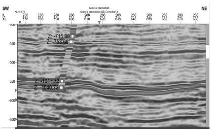
Fig. 1. Seismic section with well 73 tie. Interpreted horizons: B (blue, top of Bobrikovsky / base of Tulsky), Y (red, target Bobrikovsky reservoir), T (yellow, top of Tournaisian carbonates). Correlation coefficient = 0.85.

Three regional reflection horizons were interpreted: B (top of Bobrikovsky / base of Tulsky), Y (target horizon, top of the main sandstone reservoir), and T (top of Tournaisian carbonates). An interval velocity model (V = Vint) was built and calibrated with well tops; the depth error at wells after conversion was less than 20 cm.

Facies modeling (Truncated Gaussian Simulation)

Facies were interpreted from gamma ray and neutron porosity logs: sandstone is characterized by low GR and high neutron porosity; shale by high GR and low neutron porosity [3, 4]. Sandstone proportion from the 41 wells is 65%, shale 35%. Variogram analysis was performed on upscaled facies data [7, 9]. 

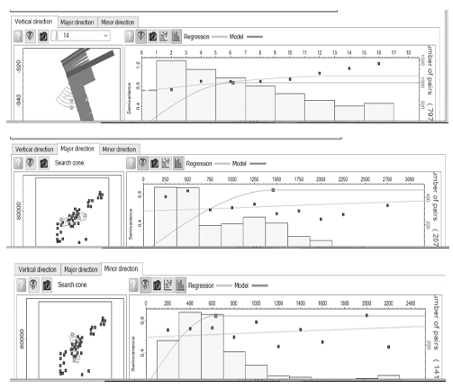
Fig. 2. Experimental variograms (blue points) and fitted theoretical spherical models (red lines): (a) vertical direction (range 6 m); (b) major direction, azimuth 75° (range 1459 m); (c) minor direction (range 630 m).

A spherical model provided the following parameters: nugget 0.1, sill 0.9, major range 1459 m (azimuth 75°), minor range 630 m, vertical range 6 m. Using these parameters, a 3D facies cube was constructed by Truncated Gaussian Simulation [7]. The model reproduces elongated sand bodies aligned with the 75° azimuth.

Seismic attributes and correlation analysis

Volumetric attributes were computed from the seismic cube; acoustic impedance (AI = ρ·Vp) was obtained by standard inversion [6, 8]. To evaluate the relationship between AI and porosity, a correlation analysis was performed at well locations intersecting horizon Y. The Pearson correlation coefficient was R = 0.61.

 

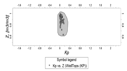
Fig. 3. Cross plot of acoustic impedance (AI) vs. well log porosity at the target horizon Y. The regression line and Pearson correlation coefficient R = 0.61 indicate a moderate positive correlation.

This value exceeds the minimum recommended threshold (0.5) for applying collocated cokriging and is statistically significant [7, 9].

Porosity modeling – collocated cokriging

Porosity was propagated using collocated cokriging, with well log porosity as the primary variable and the AI cube as the secondary variable [7, 8]. The same variogram parameters as for facies (major range 1459 m, azimuth 75°, minor range 630 m, vertical range 6 m) were used. The correlation coefficient R = 0.61 was input as a constraint. The resulting porosity cube honors well data (average absolute deviation from well log porosity = 0.5%) and shows elevated porosity (18–25%) in channel facies and lower porosity (5–12%) in floodplain and lagoonal deposits.

Fig. 4. 3D porosity cube from collocated cokriging constrained by acoustic impedance. Porosity ranges from 5% (blue) to 25% (red). The cube correctly reproduces well log values at control points and distributes porosity according to the AI trend.

Saturation modeling – Leverett J function

Oil saturation was modeled using the Leverett J function, which relates capillary pressure to rock properties. The function was calibrated to core data from the Bobrikovsky horizon with coefficients a = 0.35 and b = 2.0. The oil water contact was set at –970 m TVDSS based on regional pressure data and well logs. The J function was applied only to sandstone facies; shale and limestone were assigned zero oil saturation.

Volumetric reserve estimation

Initial geological reserves (STOIIP) were estimated by the volumetric method, summing over all grid cells above the oil water contact that belong to sandstone facies. The calculation used cell volumes, porosity, oil saturation, and a net-to-gross ratio of 1 for sandstone and 0 for shale.

Results and discussion

The facies cube contains 65% sandstone and 35% shale, with sand body orientation matching the 75° azimuth. Mean porosity from the model is 12% (range 3–25%). Validation against well data shows an average absolute deviation of 0.5%, well within petrophysical uncertainty. Average oil saturation in the oil zone is 81%, with a transition zone thickness of 2–3 m.

Reserve estimates are summarized in the Table 1.

Table 1.

Initial geological oil reserves of the Bobrikovsky horizon

Interval	Geological reserves, 10⁶ m³	Geological reserves, 10⁶ tonnes	Note
Y_corr – Turne_corr	19.8	16.8	Main oil‑bearing interval
Turne_corr – Turne_bot	5.6	4.8	Underlying interval
Total	25.0	21.3	STOIIP

 

Collocated cokriging was preferred over neural network methods because of the limited number of wells (41), which makes neural networks prone to overfitting [9]. For comparison, neural network based lithology prediction in complex terrigenous reservoirs has been demonstrated elsewhere [5]. The correlation R = 0.61 is sufficient for cokriging, although further improvement could be achieved by spectral decomposition or multi attribute regression [6, 8].

Limitations of this study include moderate well density, regional quality seismic data, and a deterministic single realization model (uncertainty analysis was not performed). Nevertheless, comprehensive validation (depth error <20 cm, consistency of the OWC, geological plausibility of property distributions) confirms that the model is suitable for practical applications such as infill well placement and dynamic reservoir simulation.

Conclusion

The main results of this study are as follows:

1. For the first time in the study area, a quantitative relationship between acoustic impedance and porosity of the Bobrikovsky horizon was established (R = 0.61), allowing AI to be used as a secondary variable in cokriging [6, 8].
2. A 3D facies model was built using Truncated Gaussian Simulation with variogram parameters (major range 1459 m, azimuth 75°) that realistically reproduces elongated sand bodies [7, 9].
3. Porosity modeling by collocated cokriging yielded a deviation of only 0.5% from well data [7, 8].
4. Oil saturation was modeled using the Leverett J function with an oil water contact at –970 m; average oil saturation in the reservoir is 81%.
5. Initial geological reserves were estimated at 25.0×10⁶ m³ (21.3×10⁶ tonnes).
6. The proposed integrated workflow is recommended for geological modeling of similar terrigenous reservoirs in the Volga Ural province [1, 3, 6].